The Invisible Menu - Part 2: The Debris Spectrum Nobody Talks About
Part 2 of the Invisible Menu blog series.
In any restaurant, what arrives at the table tells you everything about what happens in the kitchen. Order a simple salad, receive a dish contaminated with ingredients you didn't request, and you know something has gone wrong behind the scenes.
Cell samples are no different. Every sample carries uninvited guests—contaminants that corrupt data, waste resources, and undermine reproducibility. Most researchers never see the full menu of what's actually being served.
Meet the five courses you didn't order.
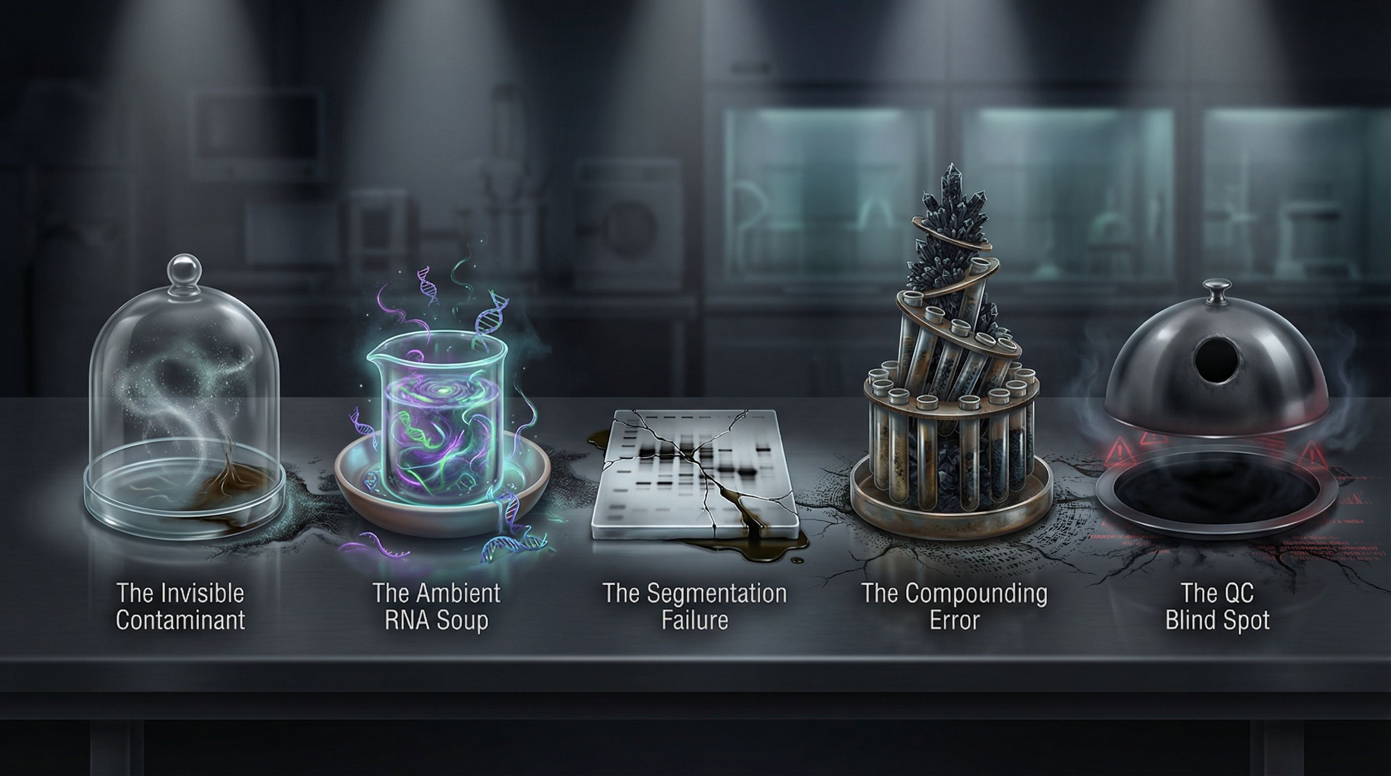
Course One: The Invisible Contaminant
Every sample preparation involves physical manipulation. Tissue gets minced. Pipettes triturate. Enzymes digest. At each step, debris particles enter the mixture—fragments of extracellular matrix, damaged cell membranes, aggregated proteins.
The Invisible Contaminant
Image-based counters exclude debris from cell counts, but they never quantify how much was excluded. A sample could be 40% debris, and as long as the algorithm correctly identifies the cells, no warning appears. The contamination remains invisible—present in every dish but absent from the menu.
Why does this matter? Because a count without context is just a number. Knowing "one million cells" means nothing if thirty percent of the sample volume is actually debris masquerading as acceptable.
Course Two: The Ambient RNA Soup
When cells die or get damaged during preparation, they release their contents into the surrounding media. This cell-free material—RNA, proteins, metabolites—creates what single-cell researchers call "the soup."
The Soup Detector Problem
In single-cell genomics, ambient RNA represents a particularly insidious contaminant. During droplet generation, this soup gets encapsulated alongside viable cells. The result? Every single-cell library carries background signal that didn't come from intact cells. Bioinformatics tools can attempt correction, but post-hoc removal always introduces uncertainty. The cleaner the sample going in, the cleaner the data coming out.
How much soup is too much? That depends on the application. But without quantifying debris levels before loading expensive chips, researchers have no way to make informed go/no-go decisions.
Course Three: The Segmentation Failure
Image-based counting relies on AI algorithms trained to identify cells and separate them from background. These algorithms have become remarkably sophisticated. But every algorithm has limitations.
The Segmentation Failure
AI segmentation algorithms fail when encountering samples they weren't trained on. Debris patterns vary. Cell clusters form unpredictably. Focus planes shift. Even in ideal conditions, image-based counting carries 3-4% error per image—errors that compound across multiple fields and propagate to downstream applications.
The fundamental challenge: imaging sees what it expects to see. When samples contain unexpected debris, unusual clustering, or focus inconsistencies, the algorithm guesses. Sometimes correctly. Often not.
Course Four: The Compounding Error
Counting errors don't exist in isolation. When fluorescence or viability stains are added to a debris-contaminated sample, the errors multiply.
Consider a sample where debris is miscounted as cells. The total count is inflated. Now add a viability stain. The debris doesn't take up the stain—it's not alive or dead in the biological sense. But the algorithm has already counted it as part of the population. The viability calculation? Fundamentally compromised.
The Multiplicative Effect
If fifty percent of your counted "cells" are actually debris, and none of that debris stains with PI, you've introduced a massive error window into viability measurements. The original counting error multiplies through every downstream calculation. One wrong ingredient corrupts the entire recipe.
Course Five: The QC Blind Spot
Every laboratory has quality control checkpoints. Sample preparation follows SOPs. Reagents are verified. Equipment is calibrated. But what about sample quality itself?
The QC Blind Spot
Most workflows lack objective debris thresholds. No standardized metrics exist for sample composition. No pass/fail criteria for contamination levels. Samples move forward based on cell counts alone—counts that tell nothing about what else is present. The QC checkpoint that matters most is the one nobody performs.
What would it mean to have a debris percentage threshold in your SOP? A preset gate that every sample must pass before proceeding? A standardized metric that every technician applies consistently?
Reading the Full Menu
These five villains—The Invisible Contaminant, The Ambient RNA Soup, The Segmentation Failure, The Compounding Error, and The QC Blind Spot—exist in every sample. They arrive uninvited. They corrupt data silently. They waste resources invisibly.
The question isn't whether they're present. They always are. The question is whether you can see them.
Key Takeaway
Five contaminants corrupt every sample. Image counters exclude them from counts but never reveal their presence. Until you can quantify what's actually in your sample—not just how many cells—these villains control the menu.
In Part 3 of The Invisible Menu, we'll examine the twist that changes everything: why the solution isn't better AI or smarter algorithms, but a fundamentally different approach to measuring what's actually there. Physics versus pixels. The truth the imaging industry doesn't want you to know.
Know Your Enemies
These five villains hide in every sample. Are you ready to see them?